Solution path of the L2E trend filtering regression with distance penalization
L2E_TF_dist.RdL2E_TF_dist computes the solution path of the robust trend filtering regression under the L2 criterion with distance penalty
L2E_TF_dist(
  y,
  X,
  beta0,
  tau0,
  D,
  kSeq,
  rhoSeq,
  max_iter = 100,
  tol = 1e-04,
  Show.Time = TRUE
)
Arguments
| y | Response vector |
|---|---|
| X | Design matrix. Default is the identity matrix. |
| beta0 | Initial vector of regression coefficients, can be omitted |
| tau0 | Initial precision estimate, can be omitted |
| D | The fusion matrix |
| kSeq | A sequence of tuning parameter k, the number of nonzero entries in D*beta |
| rhoSeq | An increasing sequence of tuning parameter rho, can be omitted |
| max_iter | Maximum number of iterations |
| tol | Relative tolerance |
| Show.Time | Report the computing time |
Value
Returns a list object containing the estimates for beta (matrix) and tau (vector) for each value of the tuning parameter k, the path of estimates for beta (list of matrices) and tau (matrix) for each value of rho, the run time (vector) for each k, and the sequence of rho and k used in the regression (vectors)
Examples
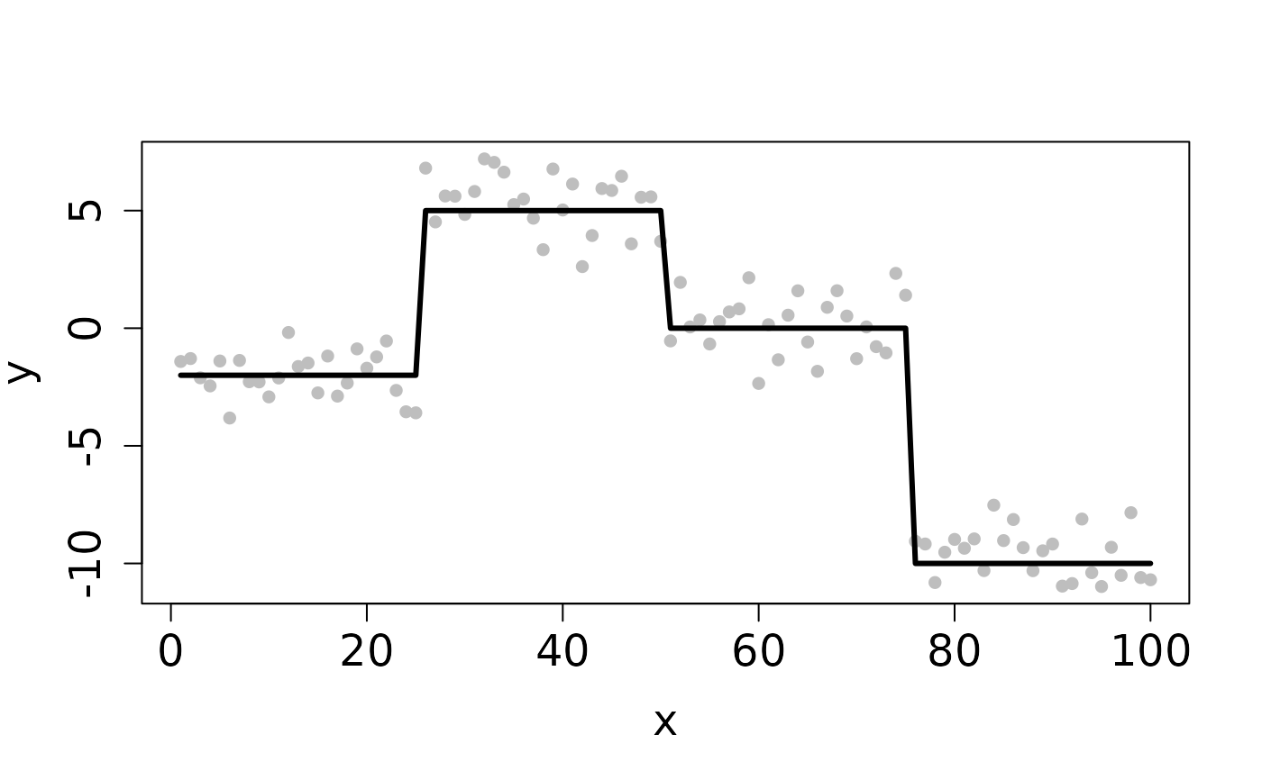
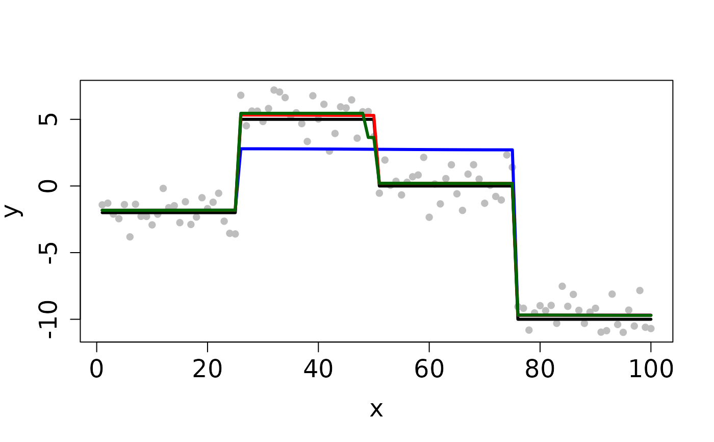
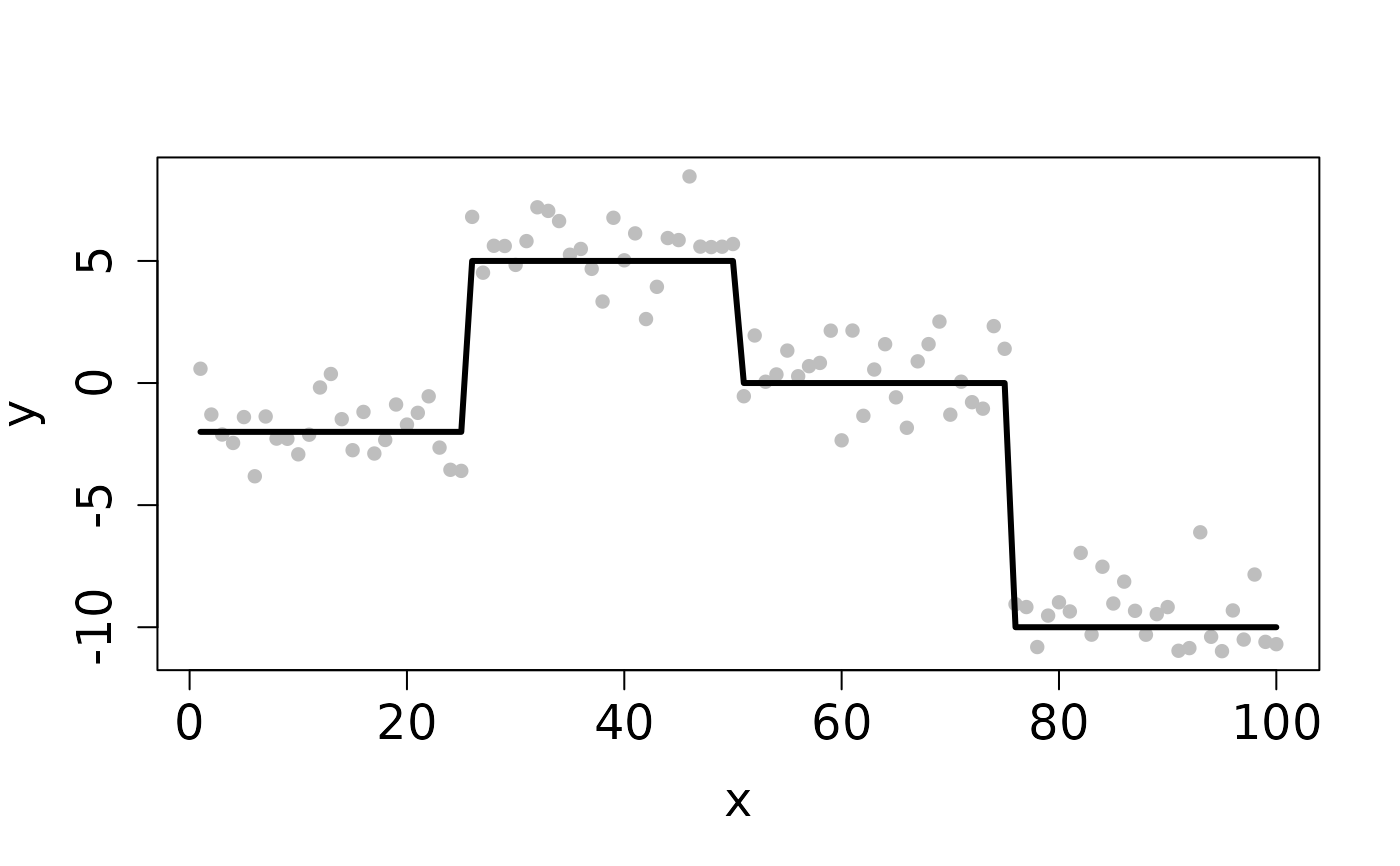
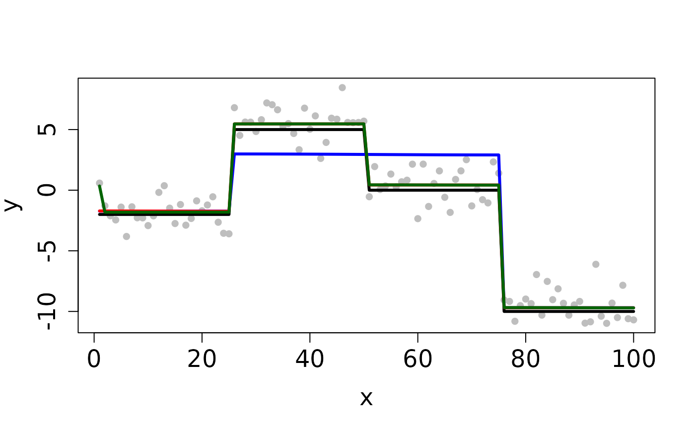
## Completes in 15 seconds set.seed(12345) n <- 100 x <- 1:n f <- matrix(rep(c(-2,5,0,-10), each=n/4), ncol=1) y <- y0 <- f + rnorm(length(f)) ## Clean Data plot(x, y, pch=16, cex.lab=1.5, cex.axis=1.5, cex.sub=1.5, col='gray')#> user system elapsed #> 0.993 0.000 0.993 #> user system elapsed #> 0.682 0.004 0.686 #> user system elapsed #> 4.006 0.000 4.008## Contaminated Data ix <- sample(1:n, 10) y[ix] <- y0[ix] + 2 plot(x, y, pch=16, cex.lab=1.5, cex.axis=1.5, cex.sub=1.5, col='gray')sol <- L2E_TF_dist(y=y, D=D, kSeq=k, rhoSeq=rho)#> user system elapsed #> 1.026 0.001 1.026 #> user system elapsed #> 0.563 0.000 0.564 #> user system elapsed #> 4.022 0.000 4.022