L2E isotonic regression - PG
l2e_regression_isotonic.Rdl2e_regression_isotonic performs L2E isotonic regression via block coordinate descent
with proximal gradient for updating both beta and tau.
l2e_regression_isotonic(
  y,
  b,
  tau,
  max_iter = 100,
  tol = 1e-04,
  Show.Time = TRUE
)
Arguments
| y | Response vector |
|---|---|
| b | Initial vector of regression coefficients |
| tau | Initial precision estimate |
| max_iter | Maximum number of iterations |
| tol | Relative tolerance |
| Show.Time | Report the computing time |
Value
Returns a list object containing the estimates for beta (vector) and tau (scalar), the number of outer block descent iterations until convergence (scalar), and the number of inner iterations per outer iteration for updating beta and tau (vectors)
Examples
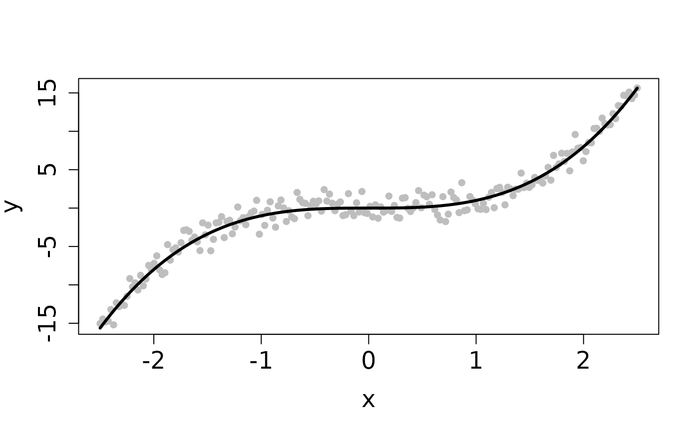
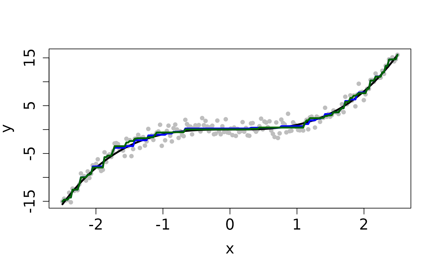
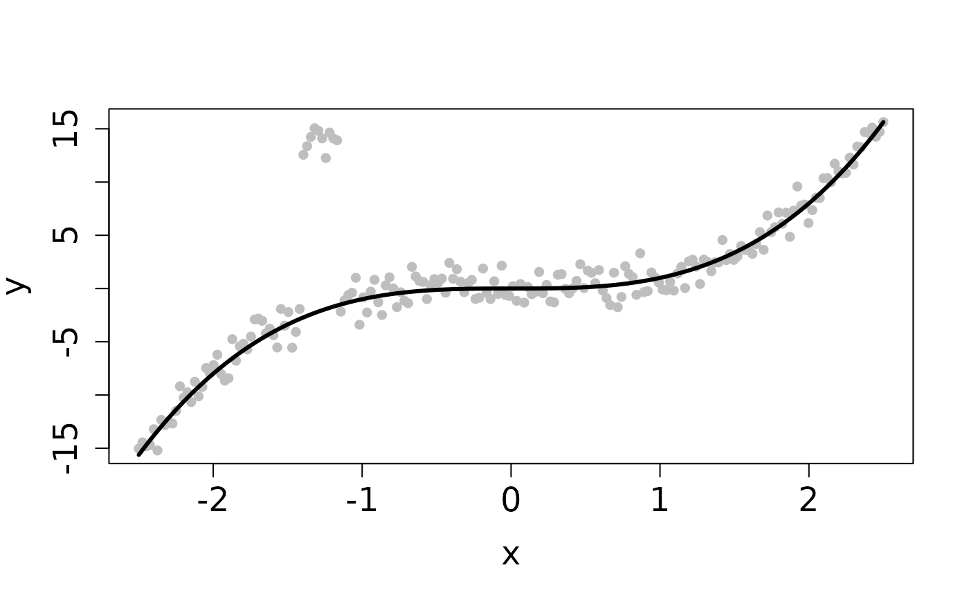
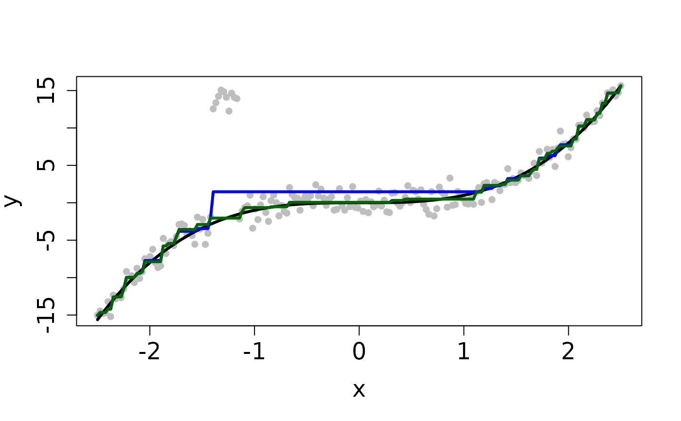
set.seed(12345) n <- 200 tau <- 1 x <- seq(-2.5, 2.5, length.out=n) f <- x^3 y <- f + (1/tau)*rnorm(n) # Clean Data plot(x, y, pch=16, cex.lab=1.5, cex.axis=1.5, cex.sub=1.5, col='gray')tau <- 1 b <- y sol <- l2e_regression_isotonic(y, b, tau)#> user system elapsed #> 0.242 0.000 0.243# Contaminated Data ix <- 0:9 y[45 + ix] <- 14 + rnorm(10) plot(x, y, pch=16, cex.lab=1.5, cex.axis=1.5, cex.sub=1.5, col='gray')tau <- 1 b <- y sol <- l2e_regression_isotonic(y, b, tau)#> user system elapsed #> 0.132 0.000 0.132